Two dimensional plot of Latent Space Joint Model output

Function to plot an object of class 'lsjm'

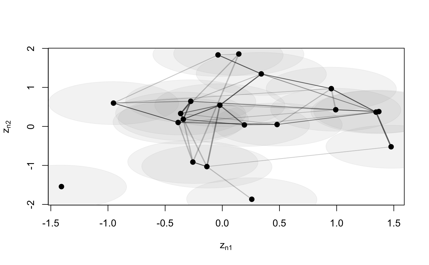
# S3 method for lsjm
plot(x, Y, drawCB = FALSE, dimZ = c(1, 2),
  plotZtilde = FALSE, colPl = 1, colEll = rgb(0.6, 0.6, 0.6, alpha =
  0.1), LEVEL = 0.95, pchplot = 20, pchEll = 19, pchPl = 19,
  cexPl = 1.1, mainZtilde = NULL, arrowhead = FALSE, curve = NULL,
  xlim = NULL, ylim = NULL, main = NULL, ...)

Arguments

x	object of class 'lsjm'
Y	list containing a (N x N) binary adjacency matrix for each network view.
drawCB	logical if drawCB = TRUE draw confidence bounds
dimZ	dimensions of the latent variable to be plotted. Default dimZ = c(1, 2)
plotZtilde	if TRUE do the plot for the last step of LSM
colPl	col for the points representing the nodes. Default colPl = NULL
colEll	col for the ellipses. Default rgb(.6, .6 ,.6 , alpha=.1)
LEVEL	levels of confidence bounds shown when plotting the ellipses. Default LEVEL = .95
pchplot	Default pchplot = 20
pchEll	pch for the ellipses. Default pchEll = 19
pchPl	pch for the points representing the nodes. Default pchPl = 19
cexPl	cex for the points representing the nodes. Default cexPl = 1.1
mainZtilde	title for single network plots TRUE do the plot for the last step of LSM
arrowhead	logical, if the arrowed are to be plotted. Default arrowhead = FALSE
curve	curvature of edges. Default curve = 0
xlim	range for x
ylim	range for y
main	main title
...	Arguments to be passed to methods, such as graphical parameters (see par).

Examples

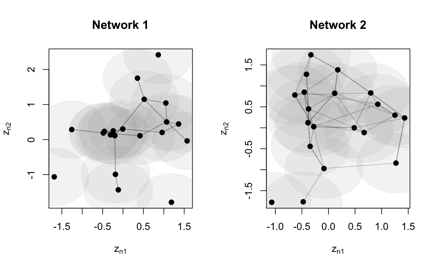
## Simulate Undirected Network
  N <- 20
  Ndata <- 2
   Y <- list()
   Y[[1]] <- network(N, directed = FALSE)[,]
   ### create a new view that is similar to the original
  for(nd in 2:Ndata){
    Y[[nd]] <- Y[[nd - 1]] - sample(c(-1, 0, 1), N * N, replace = TRUE,
    prob = c(.05, .85, .1))
    Y[[nd]] <- 1 * (Y[[nd]]  > 0 )
  diag(Y[[nd]]) <- 0
   }

par(mfrow = c(1, 2))
z <- plotY(Y[[1]], verbose = TRUE, main = 'Network 1')
plotY(Y[[2]], EZ = z, main = 'Network 2')
par(mfrow = c(1, 1))

modLSJM <- lsjm(Y, D = 2)
plot(modLSJM, Y, drawCB = TRUE)
plot(modLSJM, Y, drawCB = TRUE, plotZtilde = TRUE)