Latent Space Joint Model

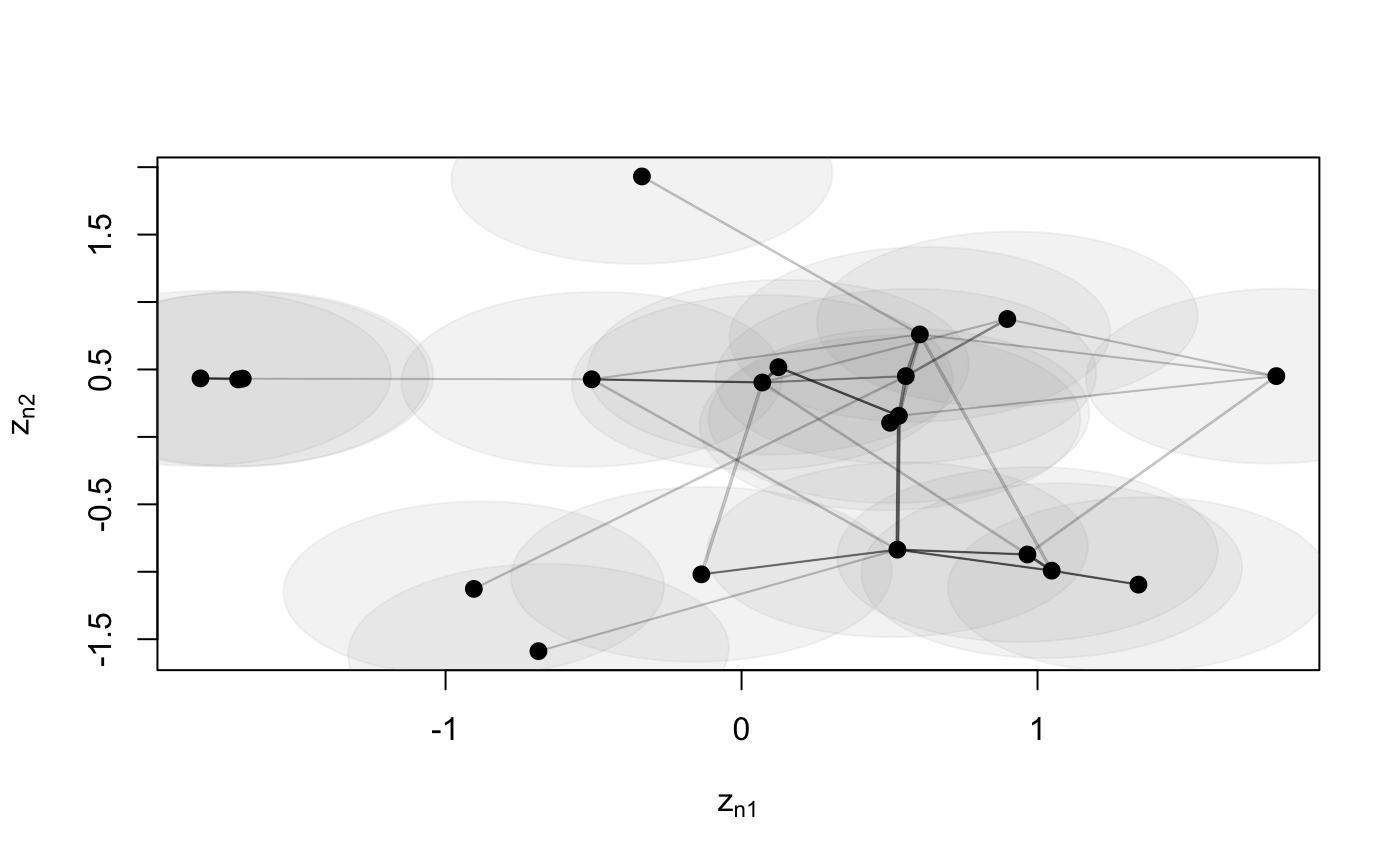
Function to joint modelling of multiple network views using the Latent Space Jont Model (LSJM) Gollini and Murphy (2016). The LSJM merges the information given by the multiple network views by assuming that the probability of a node being connected with other nodes in each view is explained by a unique latent variable.

lsjm(Y, D, sigma = 1, xi = rep(0, length(Y)), psi2 = rep(2,
  length(Y)), Niter = 500, tol = 0.1^2, preit = 20,
  randomZ = FALSE)

Arguments

Y	list containing a (N x N) binary adjacency matrix for each network view.
D	integer dimension of the latent space
sigma	(D x D) variance/covariance matrix of the prior distribution for the latent positions. Default sigma = 1
xi	vector of means of the prior distributions of \(\alpha\). Default xi = 0
psi2	vector of variances of the prior distributions of \(\alpha\). Default psi2 = 2
Niter	maximum number of iterations. Default Niter = 500
tol	desired tolerance. Default tol = 0.1^2
preit	Preliminary number of iterations default preit = 20
randomZ	logical; If randomZ = TRUE random initialization for the latent positions is used. If randomZ = FALSE and D = 2 or 3 the latent positions are initialized using the Fruchterman-Reingold method and multidimensional scaling is used for D = 1 or D > 3. Default randomZ = FALSE

Value

List containing:

• EZ (N x D) matrix containing the posterior means of the latent positions

• VZ (D x D) matrix containing the posterior variance of the latent positions

• lsmEZ list contatining a (N x D) matrix for each network view containing the posterior means of the latent positions under each model in the latent space.

• lsmVZ list contatining a (D x D) matrix for each network view containing the posterior variance of the latent positions under each model in the latent space.

• xiT vector of means of the posterior distributions of \(\alpha\)

• psi2T vector of variances of the posterior distributions of \(\alpha\)

• Ell expected log-likelihood

References

Gollini, I., and Murphy, T. B. (2016), 'Joint Modelling of Multiple Network Views', Journal of Computational and Graphical Statistics, 25(1), 246-265 http://arxiv.org/abs/1301.3759.

Examples

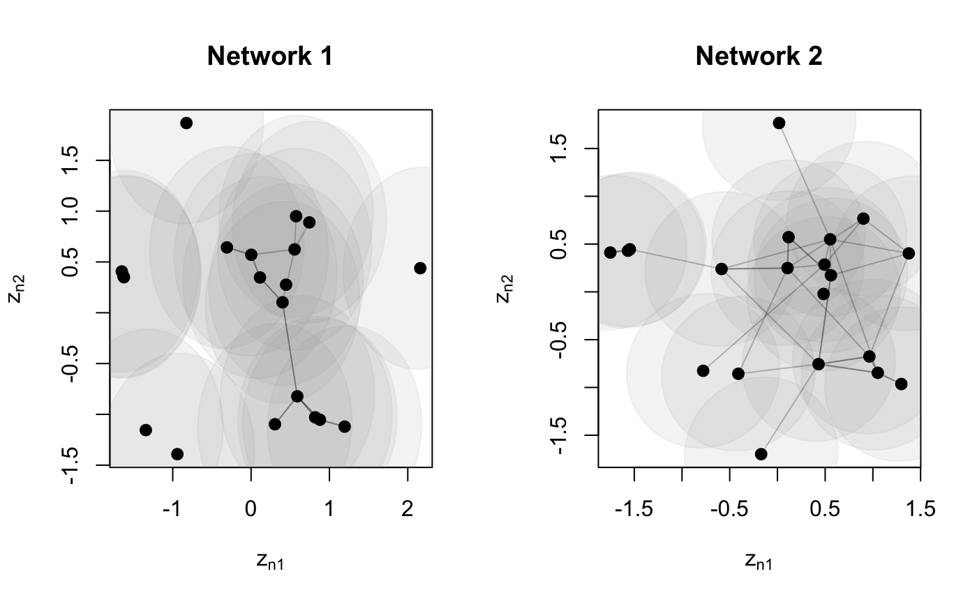
## Simulate Undirected Network
  N <- 20
  Ndata <- 2
   Y <- list()
   Y[[1]] <- network(N, directed = FALSE)[,]
   ### create a new view that is similar to the original

  for(nd in 2:Ndata){
    Y[[nd]] <- Y[[nd - 1]] - sample(c(-1, 0, 1), N * N, replace = TRUE,
   prob = c(.05, .85, .1))
    Y[[nd]] <- 1 * (Y[[nd]]  > 0 )
  diag(Y[[nd]]) <- 0
   }

par(mfrow = c(1, 2))
z <- plotY(Y[[1]], verbose = TRUE, main = 'Network 1')
plotY(Y[[2]], EZ = z, main = 'Network 2')
par(mfrow = c(1, 1))

modLSJM <- lsjm(Y, D = 2)
plot(modLSJM, Y, drawCB = TRUE)
plot(modLSJM, Y, drawCB = TRUE, plotZtilde = TRUE)