Boxplot and ROC Curves

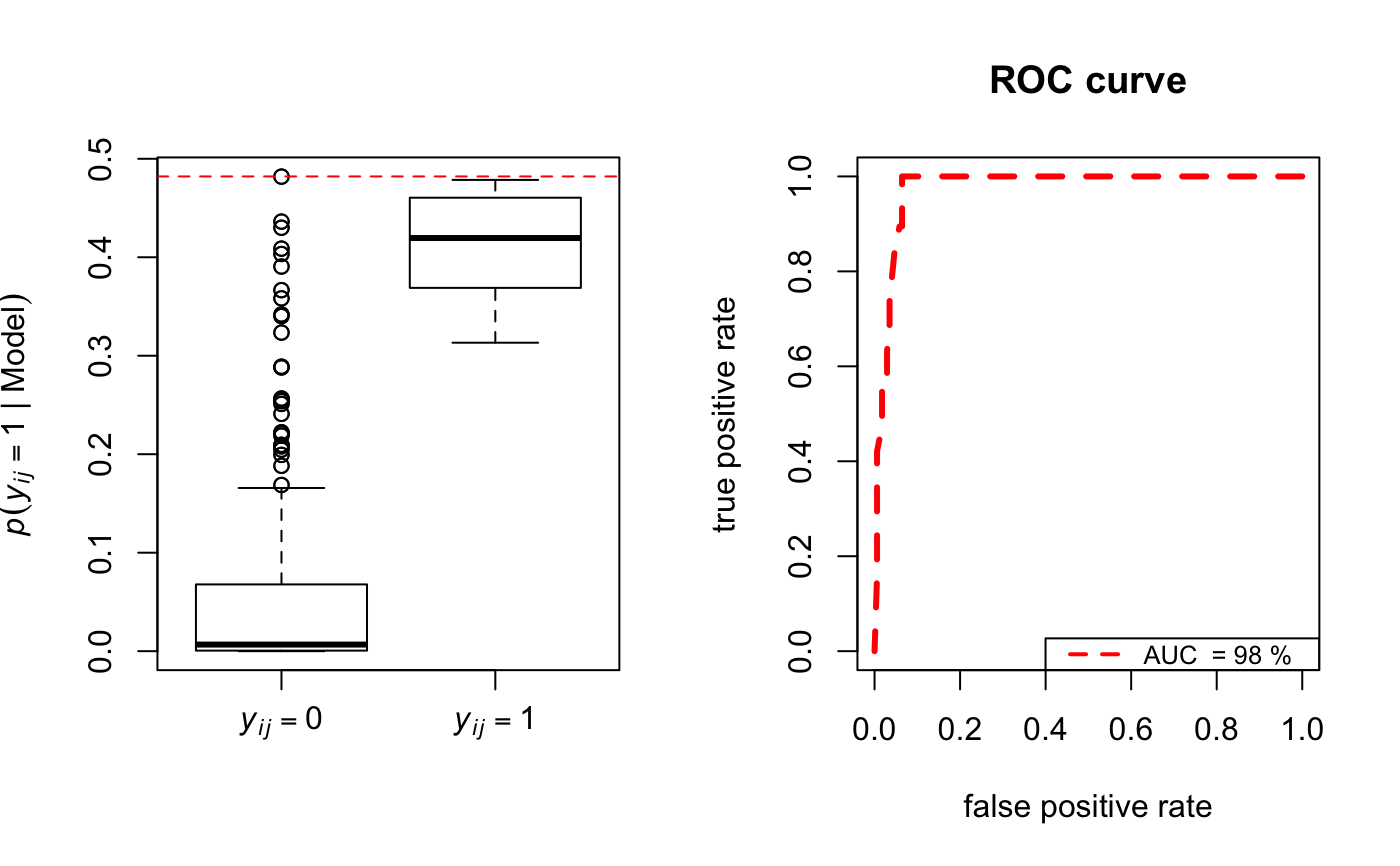
Function to display boxplots and ROC curves to show model fit in terms of in-sample link prediction.

boxroc(Y, EZ, xiT, BOXPLOT = FALSE, ROC = FALSE, Lroc = 100,
  labelsPlot = NULL, powdist = 2, cexRocLeg = 0.8, colRoc = seq(2,
  Ndata + 1), ltyRoc = seq(2, Ndata + 1), lwdRoc = 2, ...)

Arguments

Y	(N x N) binary adjacency matrix, or list containing the adjacency matrices.
EZ	(N x D) matrix (or list of matrices) containing the posterior means of the latent positions
xiT	vector of posterior means of the parameter \(\alpha\)
BOXPLOT	logical; if TRUE draws the boxplot. Default BOXPLOT = FALSE
ROC	logical; if TRUE draws the ROC curve. Default ROC = FALSE
Lroc	number of intervals in the ROC curve. Default Lroc = 100
labelsPlot	main title for the boxplot. Default labelsPlot = NULL
powdist	vector of power of the distance default powdist = 2, squared Euclidean distance, the alternative is 1, for the Euclidean distance
cexRocLeg	cex for the ROC curve. Default cexRocLeg = .8
colRoc	col for the ROC curve. Default colRoc = seq(2, Ndata + 1)
ltyRoc	lty for the ROC curve. Default ltyRoc = seq(2, Ndata + 1)
lwdRoc	lwd for the ROC curve. Default lwdRoc = 2
...	Arguments to be passed to methods, such as graphical parameters (see par).

Value

The area under the ROC curve (AUC) and the selected plots. The closer the AUC takes values to 1 the better the fit.

References

Gollini, I., and Murphy, T. B. (2016), 'Joint Modelling of Multiple Network Views', Journal of Computational and Graphical Statistics, 25(1), 246-265 http://arxiv.org/abs/1301.3759.

See also

lsm, lsjm

Examples

N <- 20
Y <- network(N, directed = FALSE)[,]

modLSM <- lsm(Y, D = 2)
bp <- boxroc(Y,
EZ = modLSM$lsmEZ,
xiT = modLSM$xiT,
Lroc = 150,
ROC = TRUE,
BOXPLOT = TRUE)
#> [1] 0.9766082

print(bp)
#> $AUC
#> [1] 0.9766082
#> 
#> $statsboxplot
#> $statsboxplot[[1]]
#>              [,1]      [,2]
#> [1,] 0.0000000000 0.3132298
#> [2,] 0.0005709753 0.3689158
#> [3,] 0.0067040780 0.4195257
#> [4,] 0.0677938491 0.4604811
#> [5,] 0.1657144271 0.4785512
#> 
#>